
Feature Engineering is a crucial step in the process of building a Machine Learning pipeline, as the features will be used by the algorithm as predictors.
Therefore, it’s advisable to prioritise building and optimizing our features to make sure that we start with a robust data model - which will result in our machine learning model achieving good results.
There are many challenges which may arise during the preparation of features. Our data starts in a specific format, but we need to change that format and convert the way the data is structured for it to be understood by the Machine Learning Algorithm.
One common problem is misunderstanding of the business use case through inexperience, which often results in the construction of weak features.
This post will concentrate on how to approach features generally and give an example of the results after we have constructed our features, and their effect on the model.
Example: Financial transactions
Our example focuses on billing and collection at a fictional utilities company.
To simplify things, we will only be discussing data based on one table. We won’t attempt to discuss the full data model as there would be multiple tables joined together making it too complex for our purposes.
Analyzing the table
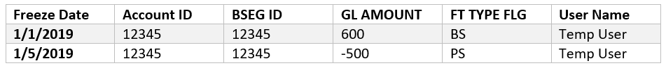
The main table we will be analyzing is the Financial Transactions Table. This table holds information on different kinds of transactions for each client. There are 6 kinds of transactions:
BS: Billing Segment
BX: Billing Segment Cancelled
PS: Payment Segment
PX: Payment Segment Cancelled
AD: Adjustment
AX: Adjustment Cancelled
Each Billing Segment ID is linked to a unique transaction so we can track the different types of transactions per Billing Segment. So, for simplification purposes, we will construct this table based on the important columns:
Business use case
Now we need to revise our business use case for us to understand how we can remodel the current data into a new model that would serve our purpose and be easily digestible by the Machine Learning Model.
Our Use Case:
Increase the frequency of On Time Payment of bills by decreasing the Collection Rate for Utilities (Electricity & Water)
Description of the Use Case:
At the beginning of each month, our company bills clients for their electricity and water consumption the previous month.
We need to improve cash flow and optimize it. Currently we have clients who are delayed on their payments, which results in peaks and valleys in the cash flow. So our target is to stabilize the cash flow.
Ideally we want clients to always pay on time, however this is not the case, and the current solution we are applying is that we send a list of “users” who are currently delayed to the collections department, starting the collection process for those users. This method has a number of flaws:
The list contains currently delayed users. We are not taking into consideration the behavioral pattern of each user in order to predict whether that user will delay or not and implement a pre-emptive collections process to minimize the delays.
This list does not take into consideration any other factors, for example: after implementing our solution, instead of the collections department getting a list of 2000 delayed users, we would send them a list of the top 1000 critical users by delayed amount, this way we can assure that we are applying our solution to the users that affect cash flow the most.
The collections process sometimes takes more than two weeks, therefore, if we can predict the users who will delay, and start the collection process, we can tackle the problem before it even arises.
Feature engineering - getting started
One of the best tricks to start our feature engineering is to look at our initial definition of the Use Case. And if it is defined correctly, we can derive our starting point (and one of the strongest features).
Our use case was:
Increase the frequency of On Time Payment of bills by decreasing the Collection Rate for Utilities (Electricity & Water)
Now from the previous use case definition we can see that we are trying to decrease the collection rate, but what is the collection rate? We define the collection rate as:
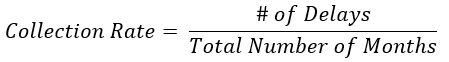
This is one of the metrics we look at and want to optimize, ideally to decrease the collection rate per user. So first we need to identify how we check if a user is eligible for collection.
The answer to that is:
If a user has not paid the bill of the previous month by the end of the current month then the user is eligible for collections.
So, for example, a user has a bill of $1,000 for January. He will receive the bill by the start of February.
If the user has not paid this bill by the end of February then the user is eligible to enter collections.
Using this knowledge, we can start to construct our new base data model, called the Cut Off Times table. This table is constructed as follows:
We have the monthly behavior of the user since he opened an account with us.
We check the account balance of that user, if it is negative or 0, this means the user does not owe us any money and is not eligible for collections, however if the balance is larger than $200 then the user is eligible to enter collections as the user is carrying more than $200 of debt over to the next month.
The structure of the Cut Off Times table is as follows:
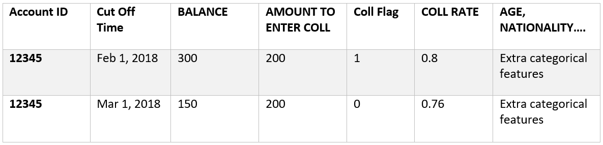
Explanation of the data in this table:
Account ID
Cut Off Time: this is the time of making the prediction
Balance: this is the sum of the account balance as of the end of the month in which the Cut Off Time falls, so if the Cut Off Time is Feb, 1 2018 then the balance is AS OF Feb, 28 2018
Amount to enter Coll: we compare the balance with this value
Coll Flag: this is the collection flag, this is = 1 if the balance exceeds the Amount to enter Coll
Coll Rate. The collection rate as of the current month. This is not taking into consideration the Coll Flag of the current month as this would cause data leakage.
Age, Nationality, Location and more: these are categorical features extracted from other data sources
Improving the data model
Now we have a solid data model, we can take this a step further and improve it. If we train the model on the current data, it might be problematic as:
The amount of data is vastly larger than required.
The model will probably over fit on the amount of details we currently have as our features are not properly engineered.
So let’s take a step back and analyze the current problem.
We have the monthly behavior (labelled by the “Coll Flag” column), however when we analyze human behavior, we do not need to put the same emphasis on all the previous months (as human behavior changes through time based on many different factors).
What we can do is start another step of reconstruction and addition of new features. The first step we can take is to aggregate the current data model on the Account ID level, this way we will compress our data massively which will result in a much faster and robust model with the pure values we want to present to our Machine Learning Model.
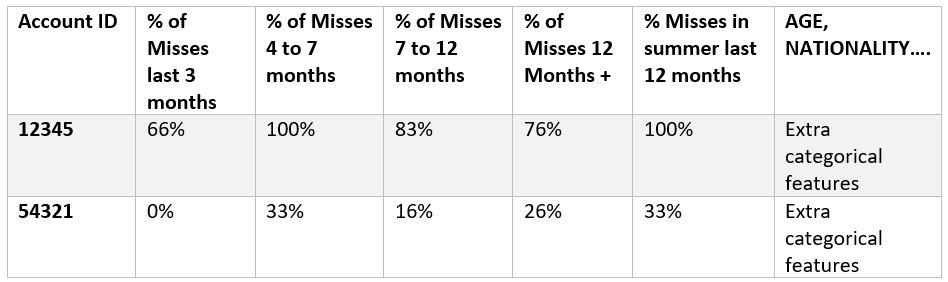
The first example of how we can Feature Engineer with emphasis on specific time durations is by turning the Coll Flag column into 4 features:
% of Misses in the past 3 months.
% of Misses from 4 to 7 months.
% of Misses from 7 to 12 months.
% of Misses from 12 Months to ∞.
And this approach has a couple of benefits:
The model will output that the most important feature out of all of those 4 features is the % of misses in the past 3 months, as it contains the most recent behavioral pattern of the user, and the farther we go back in time the less relevant it becomes. This illustrates why training on the full data without fixing the features and manually approaching this based on domain knowledge and logic will result in a weak model.
Converting this into a % will solve the problem of having a variance between users where some may have 4 years of data and some users have 2 years of data.
As you can see so far, as this is a collections problem we are concentrating on the temporal features and not so much on the categorical. However, as each user displays an individual pattern their location and nationality may also play a role.
Further improvement
Now we have a fairly robust data model, however, we can still do more. Let’s add seasonality features to further improve our model. So, we can add 4 extra features:
% of Misses in Spring in the past 12 months
% of Misses in Summer in the past 12 months
% of Misses in Fall in the past 12 months
% of Misses in Winter in the past 12 months.
These 4 features look at the previous 12 months and extracts the percentage of misses within each season. And we can customize more features based on specific countries. As we are currently doing the analysis in the United Arab Emirates, we have added cultural features such as:
% of Misses in Ramadan
% of Misses in Eid
So, we reach the following data model (sample of the features):
Results
After building our Machine Learning Model and running it on the current features, we get the following result:
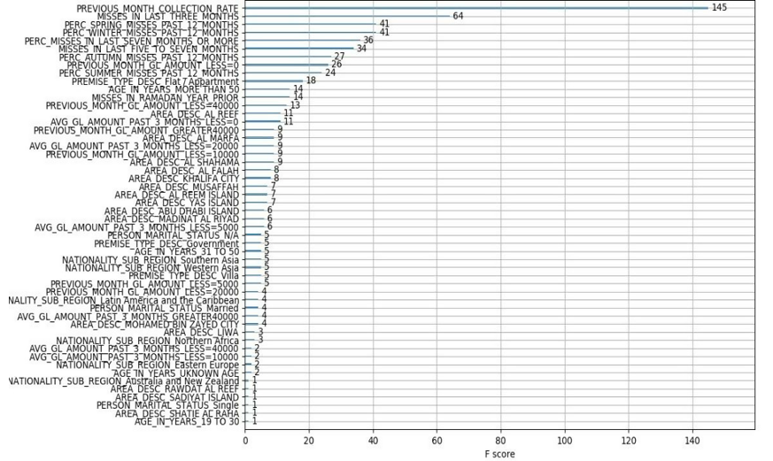
And as predicted, the strongest feature we have is the one we derived from the Use Case Definition, which is:
Previous Month Collection Rate: this feature is the collection rate AS OF the previous month.
This is followed by our hand engineered features such as:
Misses in the last 3 months
Percentage of misses in the different seasons
Misses in Ramadan/Eid
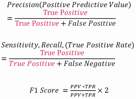
The way we calculate the relative importance of the features is by using the F1 Score:
This is just the initial step. When we work on a data science project, there is always a continuous process of improvement and testing, through multiple iterations.
When evaluating your features, remember that some features may appear to be weak or irrelevant now, but with some modifications and/or changes in the context in which they are interpreted, may turn out to be strong features which it might be useful to reincorporate later.
The most important point is to always keep an open mind and try to think outside the box when feature engineering - sometimes the least obvious answer is the key.