
SAP PA
One of the latest products that SAP has incorporated in its Business Intelligence Suite is SAP Predictive Analysis. Essentially, this product shares its main interface with SAP Lumira (formerly SAP Visual Intelligence) but the added value comes from the Predict workspace where you can find a series of algorithms to build predictive models. With these models you can display projected data behavior and trends in your visualizations, discover hidden insights and relationships in your data, among lots of other possibilities. Obviously, this proves to be very useful to make decisions based on the possible outcome of future events, or build intelligent strategies based on insights that otherwise are not clear to see. It doesn’t matter what industry a company belongs to, almost every finance department plans a budget for a fiscal year, records the actual values, and as the year progresses builds a forecast to see how the rest of the months will look like. In this article this is exactly what I will show, a very simple model to do a quick forecast based on revenue obtained in the last 5 years. The idea is that you understand the steps involved so you can build a model like this with any data series you like. At any moment you can click on the images to enlarge them.
Importing the data
Predictive Analysis supports several data sources, in this case I used a CSV file as shown below. You can also import data from excel files, Freehand SQL, Universes from BOXI 3.1 and BI4 repositories, and bring data from SAP HANA too!

Importing data from CSV file in Predictive Analysis
After importing the file, the tool heads to the Prepare workspace where you can treat the data before applying the algorithms. Here you can filter data, order data or even merge with other data sets. However, for the sake of the simplicity of this exercise I will leave it as it is and go directly to the Predict workspace.

Prepare workspace in Predictive Analysis
Build the Predictive model
In the Predict workspace, the upper sections lets you browse the different Algorithms available, use Data Preparation objects to perform additional data manipulation before or after executing the algorithms, and finally in the Data Writers tab you can write the results in database tables with JDBC drivers or in CSV files, as I will do in this case. Note that the R statistical algorithms are not enabled by default, to do so follow the steps in this article and you will have them ready in a moment.
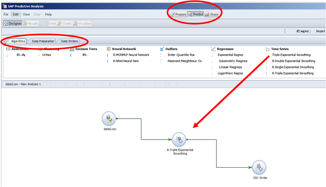
Build the Predictive Model
As you can see, my model consists of the CSV data source I defined earlier, a Time Series algorithm to do the predictive "magic" and a CSV data writer where to put the results. The following steps will focus exclusively on the predictive algorithm and the native visualization capabilities of the tool.
Configure and Execute
For this exercise, I selected the R Triple Exponential Smoothing algorithm. In short terms, this algorithm is an exponential smoothing technique that can be applied to a time series data that takes into account seasonal changes as well as trends to build forecasts. You also have simpler algorithms as the R Double Exponential Smoothing that considers the data series and its trends, as well as the R Single Exponential Smoothing algorithm that builds output based on the data series only. The selected one is the most accurate to the sample data I have in this exercise, since:
It is time series data because it has revenue per month for the last 5 years
It needs to consider seasonal changes since historically the company has obtained higher revenue in December timeframe
Also, trends are important since there are periods of the year where revenue increases or decreases
Double clicking on the algorithm opens a window where you can configure its parameters.

Configure algorith parameters
In the Primary Parameters section I set them up as follows:
The output mode is a forecast, in other cases a trend might be desired
The dependant column is Revenue since this is the variable I want to predict
Period, is the time split I desire (Months in this case)
Start Year, from when the analysis should start
Start Period, the month of the Starting Year to begin with. In this example Fiscal Years begin in April so the starting period is 4
Periods to Predict, are the number of months I want to project. Since my current Fiscal Year has only 2 closed months, I want to predict the remaining 10 months
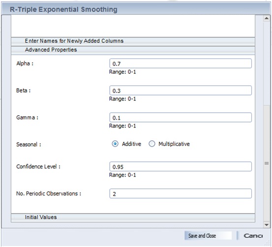
In the “Enter Names for Newly Added Columns” I simply labeled the output columns, i.e. Forecast Revenue, Years and Months. The tricky part is in the “Advanced Properties” section:

Advanced Properties
The Alpha parameter refers to a weight value that affects the data series
The Beta parameter refers to a weight value that affects the trends in the data series
The Gamma parameter refers to a weight value that affects the seasonality of the data
No. Periodic Observations means that output will be available once there are at least 2 periods (years) available. Therefore, we will start seeing predicted values from the second year onwards.
Visualize the results
After the algorithm is configured, you can hover your mouse over it and click the “Run Till Here” button to execute the model. It will notify you once the execution is done and ask to head to the Results view where we can use the visualization capabilities of SAP Predictive Analysis:
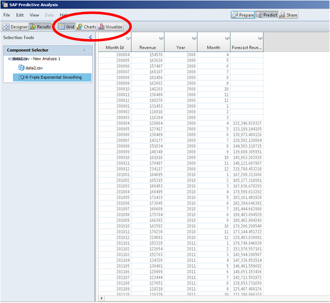
visualization capabilities of SAP Predictive Analysis
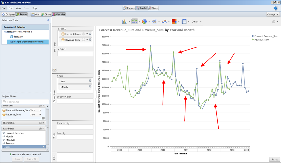
I changed from the Grid panel to the Visualize panel, where the Forecasted Revenue and the original Revenue are placed the Y axis, and the Year and Month on the X axis with a Line Chart so you can see the picture below. Do not miss the Share button to publish your visualizations!

Visualize panel
Among the first things we notice is that we don’t have forecasted values for the first year, as well as there are only forecasted values displayed for the remaining of the current Fiscal Year, both situations make absolute sense. Besides, we can see that in some periods the forecasted values are quite far from the actual values, as well as in the peak season that is December (red arrows). This is due to the weight of the Alpha/Beta/Gamma parameters. Each data series has different characteristics, so if we adjust the weight of the data series, trends and seasonality we might get more accurate results. In this case, I decide to change the weight on the data series values (Alpha parameter increased from 0.3 to 0.7); modify the trends during the year (Beta parameter increased from 0.1 to 0.3); but the seasonality will remained unchanged since I think the overall pattern is well enough. The changes are made at the Designer view in the Configuration of the algorithm as I did before.
Designer view in the Configuration of the algorithm
After I execute again, you can see how the gaps are considerably smaller. However, it is still not perfect… For example, since I increased to weight in trends the forecasted value for December 2011 went quite far from the actual one because the previous months had a significant growth, so it expected a higher value as a result. I could go on fine tuning every parameter of the algorithm to get as accurate as I can, but for now it is understood what we should try to achieve.
Visualization after changes
In summary, with a simple 30-minute exercise like this you can build a forecast based on time series data, understand the basic notions and layout of Predictive Analysis, and hopefully, many bright ideas will come to mind to use this tool in your work. Finally, you have to consider that Predictive Analysis is still in its early stages, so expect some bugs in the tool and the display (as you may have noticed in some screenshots). Nonetheless, the potential this tool has is interesting enough to not take your eyes off of it! If you have any questions or anything to add to help improve this post, please feel free to leave your comments.